What is a Function Encoder and Why Should I Care?
In the paper “Zero-Shot Reinforcement Learning via Function Encoders” (ICML 2024), I proposed an algorithm for learning basis functions for arbitrary Hilbert spaces. The paper introduces this idea and uses it to achieve zero-shot transfer in hidden-parameter system identification, multi-agent RL, and multi-task RL. However, learning basis functions is far more useful than just these fields. The purpose of this post is to introduce the idea of function encoders while a more detailed discussion on RL can be found in the paper.
What is Zero-Shot Transfer?
The entire field of machine learning is built around learning a function \(f : \mathcal{X} \to \mathcal{Y}\), where \(\mathcal{X}\) is the input space (IE an image, data on a user, the state of a system) and \(\mathcal{Y}\) is the output space (IE a scalar value, a vector, a probability). Typically a dataset \(\{x_i, f(x_i)\}_{i=1}^N\) is provided, and a neural network \(f_\theta\) is trained via gradient descent so that \(f(x_i)=f_\theta(x_i)\) for all i. Additionally, the hope is that \(f(x) \approx f_\theta(x)\) for any previously unseen \(x\). In other words, the neural network \(f_\theta\) “reproduces” \(f\).
This framework allows Netflix to predict what movies a user will like, allows Cruise to predict the future state of their autonomous vehicle, allows ChatGPT to respond to your questions, and much more. However, this framework does not fully address the messiness of real life. Consider Netflix; Their goal is to predict the rating that a user will give to a particular movie. If Netflix modeled user preferences via a single neural network, they could only predict if the average user would like a particular movie. However, every user has different preferences and their real task is to predict if a given user will like a movie. Furthermore, rather than having a single dataset of \((movie, rating)\) pairs, they have a large number of users and for each user they have a dataset of \((movie, rating)\) pairs. In other words, they have a set of datasets, where each dataset corresponds to a particular user. Their objective is to predict if a particular user will enjoy a movie, given this user’s past preferences for similar movies and the knowledge of what other similar users think. The way to understand this it that every user has an internal function mapping movies to ratings. The challenge of reproducing this function for a new user with limited amounts of data is called zero-shot transfer.
Formalizing Transfer
Consider the set of functions \(\mathcal{F} = \{f \mid f: \mathcal{X} \to \mathcal{Y} \}\). Suppose we have a set of datasets \(\mathcal{D} =\{ D_1, D_2, ...\}\) where \(D_j = \{x_i, f_j(x_i)\}_{i=1}^N\) and \(f_j \in \mathcal{F}\). This could represent the set of datasets that Netflix would have, where each \(D_j\) is data on a particular user. The goal is to learn some sort of model using \(\mathcal{D}\) so that for any unseen function \(f\), we can reproduce \(f\) during “execution” time. Of course, this requires a dataset \(D = \{x_i, f(x_i)\}_{i=1}^N\) to condition the model on at execution time. Returning to our Netflix example, this means Netflix wants to predict if a new user will like some movie given a small dataset of this user’s past preferences.
The first question is what form this model should have. The naive approach is to train a separate neural network for every function in \(\mathcal{F}\). Unfortunately, there are infinite of them, so that idea is out. Therefore, we need some sort of structure on \(\mathcal{F}\) so that a model is feasible. Suppose \(\mathcal{F}\) is a Hilbert space, which gives us some nice properties such as the continuity of the functions and the completeness of the space. Then we can reproduce every function \(f\) as a weighted combination of (orthonormal) basis functions,
\[f(x) = \sum_{i=1}^k c_i g_i(x),\quad \quad \quad[1]\]where \(g_1, g_2, ..., g_k\) are basis functions and \(c_1, c_2, ..., c_k\) are scalar coefficients (which are unique to \(f\)). This gives us a way of expressing the model. We simply need to learn the basis functions \(g_1, g_2, ..., g_k\), and find a way to compute the coefficients for any function \(f\). In theory, we may need infinite basis functions to perfectly reproduce \(f\), but in practice we are content with approximating \(f\) via a finite number of basis functions.
As mentioned, we need to compute the coefficients \(c_1, c_2, ..., c_k\) for any function \(f\), given our basis functions. Fortunately, there is an expression for this:
\[c_i = \langle f, g_i \rangle = \int_\mathcal{X} f(x)g_i(x)dx.\quad \quad \quad[2]\]Unfortunately, this is often impractical as \(\mathcal{X}\) is typically high-dimensional, and computing this integral is intractable. Furthermore, it would require exact knowledge of \(f\), which defeats the purpose of modeling it. Lastly, we only have the dataset \(D\), which gives us a few example input-output data points which are taken from \(f\). Instead, we need to approximate this integral using our small data set. Quick side note: This definition assumes the output space is scalar. If it isn’t, replace \(f(x)g_i(x)\) in the above and below equations with \(\langle f(x), g_i(x) \rangle_\mathcal{Y}\).
To approximate the inner product with a dataset, we turn to Monte Carlo integration:
\[c_i = \langle f, g_i \rangle \approx \frac{V}{N} \sum_{x_j, f(x_j) \in D}^N f(x_j) g_i(x_j),\quad \quad \quad[3]\]where \(V\) is the volume of \(\mathcal{X}\). Basically, we are approximating the integral with whatever data we happen to have. Given equation 1, we can reproduce any function with our basis functions. Given equation 3, we can compute any function’s coefficients from a small amount of data. Thus, we are able to model the space \(\mathcal{F}\). The only challenge is finding the basis functions, given the training set \(\mathcal{D}\).
Suppose we create \(k\) neural networks, each of which is a basis function. Then, we use those learned basis functions to reproduce \(f_1, f_2, ...\) via the data sets \(D_1, D_2, ...\) and equations 1 and 3. Initially, these basis functions will not span \(\mathcal{F}\), and so the basis functions will fail to reproduce \(f_1, f_2, ...\). We can measure the error of this prediction with respect to a single function \(f_j\) in the normal way (Mean squared error, cross entropy, whatever), and then we can minimize this error for all functions \(f_1, f_2, ...\) via gradient descent. This process yields an algorithm for learning basis functions for an arbitrary space \(\mathcal{F}\):
- Initialize basis functions \({𝑔_1,𝑔_2,…, 𝑔_𝑘}\) parameterized by \(\theta\)
- While not converged:
- \(𝑙𝑜𝑠𝑠=0\)
- For \(D_i \in \mathcal{D}\):
- \(𝑐_𝑖 = \langle 𝑓,𝑔_𝑖 \rangle \forall 𝑖\)
- \(\hat{f} = \sum_{i=1}^k c_i g_i\)
- \(loss = loss + \mid \mid \hat{f} - f \mid \mid ^2\)
- \(\theta = \theta - \alpha \nabla_\theta loss\)
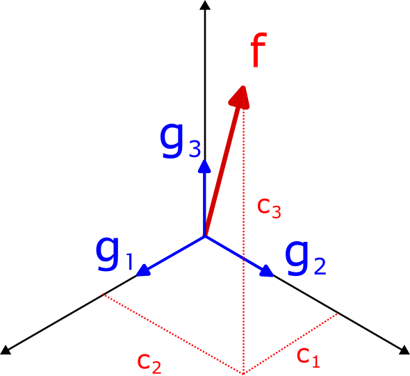
I’ve left the algorithm in terms of the inner product and vector addition/scalar multiplication terms to highlight it can be applied to any Hilbert space, so long as the basis functions are differentiable. For example, this is what it looks like applied to 3-dimensional Euclidean space:
The black arrows are the basis vectors, and the blue square indicates the 2-dimensional space \(\mathcal{F}\) that we are trying to fit. The plot on the right shows the error in reproducing vectors drawn from \(\mathcal{F}\). As you can see, the basis vectors slowly converge to spanning the space \(\mathcal{F}\). Intuitively, the same thing is happening when applying this algorithm to function spaces, where the basis functions slowly move to span the functions present in the set of datasets \(\mathcal{D}\).
When applying this algorithm to function spaces, I call the result of this algorithm a function encoder. The basis functions are typically implemented as a single neural network, with \(k\) outputs.
Examples
In this section I apply the function encoder algorithm to a few toy examples. Each is meant to illustrate the types of things you can represent with a function encoder, which I hope to show you can be applied to most problems. For more complicated problems, see my paper.
Deterministic Function Spaces
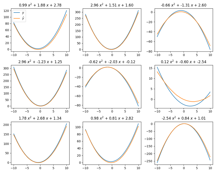
Consider trying to fit basis functions to \(\mathcal{P}_2\), the space of all quadratic functions with the form \(f(x) = ax^2 + bx + c\). The goal is to find basis functions that can reproduce any function in \(\mathcal{P}_2\) with a high degree of accuracy.
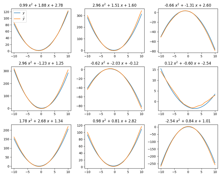
This figure shows a trained function encoder reproducing 9 different quadratic functions. To be clear, every figure is using the same basis functions. A few data points are sampled from each target (blue) function. These data points are then used to compute the coefficients via Equation 3. Then, the basis functions are used to reproduce the function via Equation 1. As you can see, the basis functions are able to accurate reproduce functions within this space.
Probability Distributions
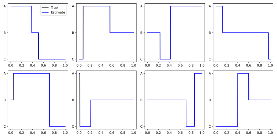
As this algorithm can be applied to any Hilbert space, we can also apply it to probability distributions. This only requires us to modify the definitions of vector addition, scalar multiplication, and the inner product. Consider a conditional discrete probability distribution, where the input space \(\mathcal{X} = [0,1]\) and the output space is three categories \(\{ A, B, C\}\). For each probability distribution, the input space is broken into three sections, each of which is assigned a category. Then, for some set of input points, we compute the correct category, and this data is used to compute the coefficients via Equation 3. Lastly, we can predict the probability of each category, conditioned on \(x\), using Equation 1. The true category is shown in black, and the category with the highest probability is shown in blue.
We can also apply this algorithm to continuous probability distributions, where the goal is to predict the probability density function for a given distribution. Again, this requires us to modify the definitions of vector addition, scalar multiplication, and the inner product, but nothing else changes. The following figure shows a function encoder’s estimate of the PDF (red) given some data points (black). Each distribution is generated via the following procedure. First sample a radius \(r\). Then sample a point along its circumference. Then sample from a Gaussian centered on that point. The resulting distribution is an infinite mixture of Gaussians. The data points shown are used to compute the coefficients, and then the coefficients are used to approximate the PDF. As you can see, the PDF closely matches the location of the data points.
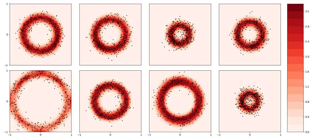
Crucially, we are estimating density without making any prior assumptions on the form of the distribution. Therefore, we can learn arbitrarily-shaped distributions using a function encoder.
Properties
Lastly, I want to highlight some useful properties of this approach.
An Expressive Representation
The coefficients of a function form a fully informative representation of the function, in the sense that the representation can be used to perfectly reproduce the function. This observation motivates the name function encoder; Any function can be encoded into a finite dimensional, fully informative representation. Furthermore, this representation has nice properties. Since it is calculated via an inner product, it is linear. This means a linear combination of functions leads to a linear combination of representations:
\[f_3 = af_1 + bf_2 \Leftrightarrow c_{f_3} = a c_{f_1} + b c_{f_2}\]This is extremely useful, as an unseen representation may still correspond to a known function due to this property. As a result, downstream tasks can more easily learn how to use this representation. Linearity also implies smoothness, so two representations that are similar are guaranteed to represent similar functions. I take advantage of this property to achieve zero-shot reinforcement learning. See the paper for more details.
Scalability!
The function encoder scales extremely well to high-dimensional function spaces. This is because the basis functions are a neural network, and the inner product is effectively a sample mean. This means it can incorporate large amounts of data with minimal overhead. In my paper, I apply this to challenging function spaces stemming from reinforcement learning problems.
Insensitivity to the Number of Basis Functions
This approach is insensitive to the number of basis functions because they are all trained as a single neural network. This means a large number of basis functions can be trained in parallel, and due to the magic of Python/Torch, this is no problem. The examples above all use \(k=100\) basis functions. This number can be increased if needed, though 100 is probably enough for most problems.
It is also possible to use less basis functions, which can be useful to get a smaller representation space. It is also possible to measure the dimensionality of a function space by decreasing the number of basis functions until performance degrades. When it degrades, this means there are not enough basis functions to fully represent the space. Even so, you often get low error anyway:
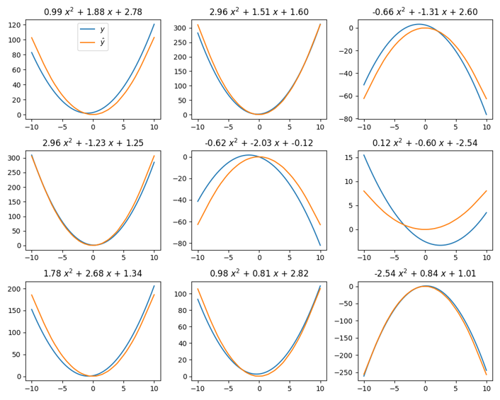
This figure shows the same quadratic example as above, but with only two basis functions. \(\mathcal{P}_2\) is a three-dimensional space, and so this is not enough basis functions. Nonetheless, the basis functions learn the best basis to explain the data. Therefore, the least important dimension, corresponding to the vertical shift, is lost, but the quadratic and linear terms are kept.
Taking this further:
Even with only one basis function, the basis still learns the quadratic term, as this is the most important term. As a result, it still gets reasonably accurate performance despite only learning a one-dimensional space. Thus, it is clear the function encoder learns the most important basis for the function space, if not enough basis functions are used. Note that “most important” corresponds to lowest loss on the training set, which is found due to the nature of gradient descent.
Zero-Shot, Online Predictions
The inner product calculation requires no expensive gradient updates. This makes it useful for online predictions. For example, suppose you modeling the dynamics of a robotic system walking on a new surface. The robot may collect a small, online data set of states, actions, and next states. This data set can be used to compute the coefficients, and then the future dynamics can be predicted right away. Crucially, the inner product is just a sample mean, and be computed extremely quickly with low memory overhead. This makes the function encoder extremely useful for online, zero-shot transfer. Furthermore, the inner product could be computed as a running sample mean, with O(1) memory overhead and O(1) compute overhead per additional data point. As a result, I expect this to be useful for low-compute, embedded systems.
One last point about coefficient calculations. Once the basis functions are trained, any method can be used to compute the coefficients. For example, given deterministic data of \(x,f(x)\) pairs, the least squares method may be used to compute the coefficients. For probability distributions, the equivalent is maximum likelihood estimation. In both cases, the goal is to find the best coefficients to explain the data. I see two main benefits of this approach. 1) The computed coefficients may be more accurate given a small dataset. 2) If the function does not lie within the learned space, least squares/maximum likelihood may give the closest representation within the learned space, IE the line connecting \(f\) and the nearest approximation will be perpendicular to the learned space. This is the best you can do for fixed basis functions. This is therefore an avenue for generalization outside of the learned function space, though these calculations are slightly more expensive (least squares) to much more expensive (maximum likelihood) than the inner product calculation.
Fin
Thanks for taking the time to read my post. I hope you have been convinced of the potential of this approach. If you have questions or want to chat about research, email me tyleringebrand@utexas.edu.